Overview
ctdR identifies chemicals significantly associated with a set of genes using data from the Comparative Toxicogenomics Database (CTD).
Four enrichment methods are supported through a single
enrichment_CTD() interface; the input shape depends on the
method:
-
ORA (Over-Representation Analysis) – gene list +
hypergeometric test, computed directly on
stats::phyper. -
GSEA (Gene Set Enrichment Analysis) – ranked gene
list + permutation test. Powered by
fgsea::fgsea. -
CAMERA (competitive gene-set test) – expression
matrix or
SummarizedExperiment+ design + contrast. Corrects for inter-gene correlation within each chemical’s gene set. Powered bylimma::camera. -
GSVA (Gene Set Variation Analysis) – expression
matrix or
SummarizedExperiment+ per-sample scoring. Returns chemical x sample scores in the same container it was given. Powered byGSVA::gsva.
Data licensing disclaimer
This package does NOT bundle, redistribute, or embed any data from the Comparative Toxicogenomics Database. CTD data are created and maintained by NC State University and are subject to specific licensing terms. Users must download the data directly from https://ctdbase.org and comply with the CTD Terms of Service.
Installation
ctdR has been accepted into Bioconductor. For now it is available only in Bioconductor devel (3.24); after the next Bioconductor release it will be installable from the standard (release) repository.
From Bioconductor devel (current installation method)
if (!require("BiocManager", quietly = TRUE))
    install.packages("BiocManager")
BiocManager::install(version = "devel")
BiocManager::install("ctdR")
From Bioconductor release (after the next Bioconductor release)
BiocManager::install("ctdR")Quick start
The ctdR workflow has three steps:
- Download the CTD data file (once, manually)
- Import the data into ctdR (once)
- Analyse your gene list (as many times as needed)
Step 1 – Download CTD data
Download CTD_chem_gene_ixns.csv.gz from
https://ctdbase.org/reports/CTD_chem_gene_ixns.csv.gz.
Then decompress it:
This produces CTD_chem_gene_ixns.csv (several GB
uncompressed).
Step 2 – Import into ctdR
In production you would run:
library(ctdR)
import_CTD("~/Downloads/CTD_chem_gene_ixns.csv")
For this vignette we use a small synthetic dataset bundled with the package:
library(ctdR)
sample_file <- system.file(
    "extdata", "CTD_chem_gene_ixns_sample.csv",
    package = "ctdR"
)
import_CTD(sample_file)
#> Reading CTD chemical-gene interactions from: /home/runner/work/_temp/Library/ctdR/extdata/CTD_chem_gene_ixns_sample.csv
#> Filtered to 86 human interactions
#> Mapping genes for 10 chemicals...
#> Warning: 10 ChemicalID(s) appear with more than one ChemicalName in the CTD
#> file; only the first name per ID is retained. Affected IDs: D000082, D001564,
#> D002104, D003907, D004958 ... (and 5 more)
#> CTD data cached successfully in: /tmp/RtmpwQBEev/file1e888d0097f
#>   10 chemicals | 17 unique genes | 1 s
#>   CTD release: Mon Jan 01 00:00:00 EST 2024
import_CTD() performs the following:
- Reads the CSV (skipping the 27 CTD header lines).
- Filters interactions to Homo sapiens only (OrganismID 9606).
- Collects Entrez gene IDs for each chemical.
- Maps Entrez IDs to HGNC gene symbols via
org.Hs.eg.db. - Caches the processed data locally via
BiocFileCache(undertools::R_user_dir("ctdR", "cache")).
This step takes several minutes with the full CTD file. You only need to run it once – or again when you download a newer CTD release.
Which CTD release did I use?
CTD is re-released continuously and its downloads are not versioned
in the filename: two copies of CTD_chem_gene_ixns.csv
months apart are indistinguishable from the outside. The release date
lives inside the file, on the # Report created: line of its
header, and it is the only thing that identifies which snapshot a result
came from.
import_CTD() reads that line, reports it, and keeps it.
Every result then carries it, so an analysis can state the version of
the data behind it without anyone having to remember:
# With no argument: what is in the cache right now.
ctd_provenance()
#> CTD provenance
#>   Report created: Mon Jan 01 00:00:00 EST 2024
#>   Source:         /home/runner/work/_temp/Library/ctdR/extdata/CTD_chem_gene_ixns_sample.csv
#>   Imported:       2026-10-07 06:48:56 UTC
#>   Retained:       10 chemicals, 86 chemical-gene pairs
#>   ctdR version:   0.99.11
Every result carries the same record, so you can also ask an object
you are about to report on:
ctd_provenance(ora_results).
The record holds the CTD release date, where the file came from, when you imported it, how much of it was kept, and the ctdR version. Release date and import date answer different questions and are both recorded: the first says which data, the second says when you took it.
Use ctd_provenance() rather than reaching into the
object, because the record is stored wherever the container provides
room for it. Results that carry a metadata() slot keep it
there, which is the case for the SummarizedExperiment
returned by GSVA and for a CTDFile read with
import(); the data frames from ORA, GSEA and CAMERA keep it
in an attribute. The accessor hides the difference.
The record follows subsetting, ordering, head() and the
usual dplyr verbs. It does not follow
merge() or subset(), which drop attributes;
ctd_provenance() warns rather than quietly reporting
nothing, so take the record before those if you need it after.
Step 3 – Run enrichment analysis
Prepare your gene list
Your input must be a data frame with at least two columns:
| Column | Description |
|---|---|
EntrezID |
Character or numeric Entrez gene IDs |
| (2nd column) | Numeric value per gene (e.g. p-value) |
The second column is used for ranking in GSEA and is ignored in ORA.
genes <- data.frame(
    EntrezID = c(
        "7124", "3569", "7157", "672", "1956",
        "4609", "3845", "207", "5290", "3553"
    ),
    pvalue = c(
        0.001, 0.003, 0.005, 0.008, 0.01,
        0.02, 0.03, 0.04, 0.05, 0.06
    )
)
Shared output schema
All three data-frame-returning methods (ORA, GSEA, CAMERA) share the
same leading columns. This makes it trivial to combine
results across methods (e.g. dplyr::bind_rows() on a list
of result frames).
| Column | Type | Description |
|---|---|---|
ChemicalID |
character | CTD chemical identifier |
ChemicalName |
character | Human-readable chemical name |
Method |
character | One of "ORA", "GSEA",
"CAMERA"
|
PValue |
numeric | Raw p-value from the underlying method |
PValueAdjusted |
numeric | Multiple-testing-corrected p-value (pAdjustMethod) |
Method-specific extras follow these front columns and differ by
method (documented in the sub-sections below). Rows are sorted by
PValueAdjusted ascending.
Over-Representation Analysis (ORA)
ORA tests whether the overlap between your gene list and each chemical’s known gene targets is significantly larger than expected by chance.
ora_results <- enrichment_CTD(genes, method = "ORA")
#> background: all 17 genes in the CTD sets, because no 'universe' was given. If your experiment could only detect some of them, pass those as 'universe': a background wider than what was measurable makes p-values too small.
head(ora_results)
#>   ChemicalID     ChemicalName Method      PValue PValueAdjusted GeneRatio
#> 1    D000082    Acetaminophen    ORA 0.003393665     0.03393665     10/10
#> 2    D002945        Cisplatin    ORA 0.017533937     0.08766968      9/10
#> 3    D001564   Benzo(a)pyrene    ORA 0.052241876     0.17413959      8/10
#> 4    D002104          Cadmium    ORA 0.217811600     0.54452900      6/10
#> 5    D001151          Arsenic    ORA 0.646133278     0.98663102      6/10
#> 6    D003520 Cyclophosphamide    ORA 0.685520362     0.98663102      3/10
#>   BackgroundRatio                                     EnrichedGenes Count
#> 1           12/17 TNF/IL6/TP53/BRCA1/EGFR/MYC/KRAS/AKT1/PIK3CA/IL1B    10
#> 2           11/17      TNF/IL6/TP53/BRCA1/EGFR/MYC/KRAS/AKT1/PIK3CA     9
#> 3           10/17           TNF/TP53/EGFR/MYC/KRAS/AKT1/PIK3CA/IL1B     8
#> 4            8/17                     TNF/IL6/TP53/AKT1/PIK3CA/IL1B     6
#> 5           10/17                       TNF/IL6/TP53/EGFR/KRAS/AKT1     6
#> 6            5/17                                    TP53/BRCA1/MYC     3
#>   FoldEnrichment
#> 1       1.416667
#> 2       1.390909
#> 3       1.360000
#> 4       1.275000
#> 5       1.020000
#> 6       1.020000
ORA method-specific columns (in addition to the shared schema above):
| Column | Description |
|---|---|
GeneRatio |
Proportion of input genes in the set |
BackgroundRatio |
Background ratio |
FoldEnrichment |
GeneRatio / BackgroundRatio |
EnrichedGenes |
Enriched gene symbols (comma-separated) |
Count |
Number of overlapping genes |
Gene Set Enrichment Analysis (GSEA)
GSEA uses the full ranked gene list to detect chemicals whose targets
cluster toward the top or bottom of the ranking. For best results,
supply a signed ranking statistic (e.g. the moderated t-statistic from
limma::eBayes()) as a column named stat. When
stat is absent, ctdR falls back to
-log10(pvalue), which loses directionality and may produce
ties.
# Quick-start: no signed statistic available in this
# toy gene list, so the pvalue fallback is used.
gsea_results <- enrichment_CTD(genes, method = "GSEA")
#> Warning: GSEA: no 'stat' column found in input. Falling back to -log10(second
#> column) for ranking, which loses directionality and may produce ties at
#> non-significant genes. Add a signed ranking statistic (e.g. the moderated
#> t-statistic from limma::eBayes()) as a column named 'stat' to suppress this
#> warning.
#> Warning in prepareStats(stats, scoreType, gseaParam): All values in the stats
#> vector are greater than zero and scoreType is "std", maybe you should switch to
#> scoreType = "pos".
head(gsea_results)
#>   ChemicalID  ChemicalName Method     PValue PValueAdjusted    log2err
#> 1    D003907 Dexamethasone   GSEA 0.05477308      0.2347418 0.24133998
#> 2    D008687     Metformin   GSEA 0.07183908      0.2347418 0.28785712
#> 3    D014635 Valproic Acid   GSEA 0.07824726      0.2347418 0.19991523
#> 4    D002104       Cadmium   GSEA 0.13411079      0.3017493 0.14375899
#> 5    D002945     Cisplatin   GSEA 0.20100503      0.3618090 0.12384217
#> 6    D001151       Arsenic   GSEA 0.32507289      0.4084507 0.08528847
#>   EnrichmentScore NormalizedEnrichmentScore GeneSetSize  LeadingEdge
#> 1       0.8188439                  1.562933           3   7124, 3569
#> 2      -0.8000000                 -1.704845           5 3553, 52....
#> 3       0.7980094                  1.523166           3   7124, 3569
#> 4       0.6661635                  1.319611           6 7124, 35....
#> 5       1.0000000                  1.244519           9 7124, 35....
#> 6       0.6138938                  1.216069           6 7124, 35....
#>                                          EnrichedGenes
#> 1                                       TNF, IL6, IL1B
#> 2                        EGFR, MYC, AKT1, PIK3CA, IL1B
#> 3                                       TNF, IL6, AKT1
#> 4                   TNF, IL6, TP53, AKT1, PIK3CA, IL1B
#> 5 TNF, IL6, TP53, BRCA1, EGFR, MYC, KRAS, AKT1, PIK3CA
#> 6                     TNF, IL6, TP53, EGFR, KRAS, AKT1
GSEA method-specific columns (in addition to the shared schema above):
| Column | Description |
|---|---|
EnrichmentScore |
Enrichment score (ES from fgsea) |
NormalizedEnrichmentScore |
Normalized enrichment score (NES from fgsea): the
enrichment score scaled for gene set size. This is the quantity to
compare between chemicals |
GeneSetSize |
Size of the gene set used |
LeadingEdge |
Leading-edge gene subset |
EnrichedGenes |
Comma-separated enriched genes |
End-to-end example with real RNA-seq data (GSE311566)
The hand-coded genes data frame above is convenient for
the Quick start but does not exercise the matrix-based methods. This
section ties everything together on a small subset of GEO
GSE311566 – human PBMCs treated with dexamethasone
vs vehicle (DMSO) in female donors. The bundled subset
inst/extdata/GSE311566_subset.rds contains 1,500
top-variance genes (plus the 17 genes referenced by the toy CTD sample),
log2-transformed normalised counts, 7 samples total (4 DMSO + 3 Dex).
See inst/extdata/README.md for provenance.
It is stored as a SummarizedExperiment,
the standard Bioconductor container for assay data: the expression
matrix and the sample annotation live in one object, so subsetting or
reordering samples moves both together and cannot silently desynchronise
the group labels from the columns they describe.
library(SummarizedExperiment)
#> Loading required package: MatrixGenerics
#> Loading required package: matrixStats
#>
#> Attaching package: 'MatrixGenerics'
#> The following objects are masked from 'package:matrixStats':
#>
#>     colAlls, colAnyNAs, colAnys, colAvgsPerRowSet, colCollapse,
#>     colCounts, colCummaxs, colCummins, colCumprods, colCumsums,
#>     colDiffs, colIQRDiffs, colIQRs, colLogSumExps, colMadDiffs,
#>     colMads, colMaxs, colMeans2, colMedians, colMins, colOrderStats,
#>     colProds, colQuantiles, colRanges, colRanks, colSdDiffs, colSds,
#>     colSums2, colTabulates, colVarDiffs, colVars, colWeightedMads,
#>     colWeightedMeans, colWeightedMedians, colWeightedSds,
#>     colWeightedVars, rowAlls, rowAnyNAs, rowAnys, rowAvgsPerColSet,
#>     rowCollapse, rowCounts, rowCummaxs, rowCummins, rowCumprods,
#>     rowCumsums, rowDiffs, rowIQRDiffs, rowIQRs, rowLogSumExps,
#>     rowMadDiffs, rowMads, rowMaxs, rowMeans2, rowMedians, rowMins,
#>     rowOrderStats, rowProds, rowQuantiles, rowRanges, rowRanks,
#>     rowSdDiffs, rowSds, rowSums2, rowTabulates, rowVarDiffs, rowVars,
#>     rowWeightedMads, rowWeightedMeans, rowWeightedMedians,
#>     rowWeightedSds, rowWeightedVars
#> Loading required package: GenomicRanges
#> Loading required package: stats4
#> Loading required package: BiocGenerics
#> Loading required package: generics
#>
#> Attaching package: 'generics'
#> The following objects are masked from 'package:base':
#>
#>     as.difftime, as.factor, as.ordered, intersect, is.element, setdiff,
#>     setequal, union
#>
#> Attaching package: 'BiocGenerics'
#> The following objects are masked from 'package:stats':
#>
#>     IQR, mad, sd, var, xtabs
#> The following objects are masked from 'package:base':
#>
#>     anyDuplicated, aperm, append, as.data.frame, basename, cbind,
#>     colnames, dirname, do.call, duplicated, eval, evalq, Filter, Find,
#>     get, grep, grepl, is.unsorted, lapply, Map, mapply, match, mget,
#>     order, paste, pmax, pmax.int, pmin, pmin.int, Position, rank,
#>     rbind, Reduce, rownames, sapply, saveRDS, table, tapply, unique,
#>     unsplit, which.max, which.min
#> Loading required package: S4Vectors
#>
#> Attaching package: 'S4Vectors'
#> The following object is masked from 'package:utils':
#>
#>     findMatches
#> The following objects are masked from 'package:base':
#>
#>     expand.grid, I, unname
#> Loading required package: IRanges
#> Loading required package: Seqinfo
#> Loading required package: Biobase
#> Welcome to Bioconductor
#>
#>     Vignettes contain introductory material; view with
#>     'browseVignettes()'. To cite Bioconductor, see
#>     'citation("Biobase")', and for packages 'citation("pkgname")'.
#>
#> Attaching package: 'Biobase'
#> The following object is masked from 'package:MatrixGenerics':
#>
#>     rowMedians
#> The following objects are masked from 'package:matrixStats':
#>
#>     anyMissing, rowMedians

se <- readRDS(system.file(
    "extdata", "GSE311566_subset.rds", package = "ctdR"
))
se
#> class: SummarizedExperiment
#> dim: 1514 7
#> metadata(5): source url subset assay_units generated_by
#> assays(1): logcounts
#> rownames(1514): 1956 207 ... 124599 54453
#> rowData names(0):
#> colnames(7): Ctrl_F_1.counts.out Ctrl_F_2.counts.out ...
#>   DEX_F_2.counts.out DEX_F_3.counts.out
#> colData names(2): sample group
table(se$group)
#>
#> DMSO  Dex
#>    4    3
The assay is reached with assay(se) and the sample
annotation with colData(se), or with the
se$column shorthand used below.
We compute a deliberately minimal per-gene differential expression
with base R only: a two-sample t.test per gene with
BH-adjusted p-values. Production analyses should use limma,
DESeq2, or edgeR for proper count-based
modelling; this ascetic version keeps the example self-contained.
expr <- assay(se)
grp  <- se$group

de <- t(apply(expr, 1, function(y) {
    tt <- stats::t.test(y ~ grp)
    c(log2FC = unname(diff(tt$estimate)),
      pvalue = tt$p.value)
}))
de <- as.data.frame(de)
de$padj <- stats::p.adjust(de$pvalue, method = "BH")
de$EntrezID <- rownames(de)
de <- de[, c("EntrezID", "log2FC", "pvalue", "padj")]
head(de[order(de$padj), ])
#>            EntrezID    log2FC       pvalue        padj
#> 2289           2289  2.886037 1.134374e-06 0.001717442
#> 356             356 -4.028071 4.684751e-06 0.003546357
#> 105371773 105371773 -3.057902 1.153655e-05 0.005822112
#> 55301         55301  7.292765 1.673937e-05 0.006335851
#> 2833           2833 -2.936870 2.215244e-05 0.006707758
#> 7098           7098 -3.119787 4.259995e-05 0.010749388
c(padj_lt_05 = sum(de$padj < 0.05),
  pvalue_lt_05 = sum(de$pvalue < 0.05))
#>   padj_lt_05 pvalue_lt_05
#>           37          406
Real-data GSEA
GSEA uses the full ranked gene list and tends to surface the expected
chemical (Dexamethasone) near the top even with this small DE. We supply
log2FC as the stat column so that direction
(up/down) is preserved in the ranking.
gsea_real <- enrichment_CTD(
    data.frame(EntrezID = de$EntrezID,
               pvalue   = de$pvalue,
               stat     = de$log2FC),
    method = "GSEA"
)
head(gsea_real[, c("ChemicalID", "ChemicalName",
                   "PValue", "PValueAdjusted",
                   "NormalizedEnrichmentScore")])
#>   ChemicalID   ChemicalName     PValue PValueAdjusted NormalizedEnrichmentScore
#> 1    D000082  Acetaminophen 0.08121827      0.2146341                  1.478392
#> 2    D001151        Arsenic 0.10731707      0.2146341                  1.396534
#> 3    D001564 Benzo(a)pyrene 0.10731707      0.2146341                  1.396534
#> 4    D002945      Cisplatin 0.08816121      0.2146341                  1.413316
#> 5    D003907  Dexamethasone 0.10551559      0.2146341                  1.446729
#> 6    D002104        Cadmium 0.18912530      0.3152088                  1.277090
Real-data ORA
ORA is statistically meaningful only with the full CTD
download (~16,000 chemicals × millions of gene interactions,
available at https://ctdbase.org/reports/CTD_chem_gene_ixns.csv.gz).
The bundled CTD_chem_gene_ixns_sample.csv covers 10
chemicals × 17 genes — its sole purpose is API demonstration. With only
7 samples and a universe this small, ORA is expected to return zero
enriched chemicals. Set is_subset <- FALSE in the chunk
below to run a fully powered analysis on the real CTD. All other methods
(GSEA, CAMERA, GSVA) work correctly with the bundled data.
## Set is_subset <- FALSE to run ORA on the full CTD download.
## Requires CTD_chem_gene_ixns.csv.gz from ctdbase.org, decompressed locally.
is_subset <- TRUE
sig <- de[de$pvalue < 0.05, c("EntrezID", "pvalue")]

if (is_subset) {
    ora_real <- enrichment_CTD(sig, method = "ORA")
    if (nrow(ora_real)) {
        head(ora_real[, c("ChemicalID", "ChemicalName",
                          "PValue", "PValueAdjusted", "Count")])
    } else {
        message(
            "ORA returned 0 results on the toy CTD sample (expected).\n",
            "Set is_subset <- FALSE and provide CTD_chem_gene_ixns.csv",
            " for a powered analysis."
        )
    }
} else {
    ## Full CTD path -----------------------------------------------------------
    ## 1. Download https://ctdbase.org/reports/CTD_chem_gene_ixns.csv.gz
    ## 2. gunzip CTD_chem_gene_ixns.csv.gz
    ## 3. Set ctd_path to the decompressed file location
    ctd_path <- "~/Downloads/CTD_chem_gene_ixns.csv"  # adjust to your path
    import_CTD(ctd_path)
    ora_full <- enrichment_CTD(sig, method = "ORA")
    if (nrow(ora_full)) {
        head(ora_full[order(ora_full$PValue),
                      c("ChemicalID", "ChemicalName",
                        "PValue", "PValueAdjusted",
                        "FoldEnrichment", "Count")])
    } else {
        message("No chemicals enriched — check CTD file path and gene list.")
    }
}
#> background: all 17 genes in the CTD sets, because no 'universe' was given. If your experiment could only detect some of them, pass those as 'universe': a background wider than what was measurable makes p-values too small.
#>   ChemicalID     ChemicalName    PValue PValueAdjusted Count
#> 1    D000082    Acetaminophen 0.8088235              1     2
#> 2    D001151          Arsenic 0.9485294              1     1
#> 3    D001564   Benzo(a)pyrene 0.6397059              1     2
#> 4    D002104          Cadmium 0.4529412              1     2
#> 5    D002945        Cisplatin 0.7279412              1     2
#> 6    D003520 Cyclophosphamide 0.6764706              1     1
CAMERA (competitive test with inter-gene correlation)
CAMERA tests, for each chemical, whether its target genes show a stronger differential signal than the rest of the transcriptome, while correcting for inter-gene correlation within the gene set.
Unlike ORA or GSEA, CAMERA does not take a
pre-computed list of differentially expressed genes. Its inputs are the
full expression data (all genes by all samples),
supplied either as a matrix or as a SummarizedExperiment,
together with a design matrix and a
contrast: CAMERA fits the differential
model and computes the test internally. The chemical-to-gene
mapping (the gene-set “index”, built by ctdR from CTD
targets intersected with rownames(x)) is handled for you.
Note that design and contrast are two distinct
inputs: design (e.g. model.matrix(~ se$group))
describes the whole experimental layout, intercept plus any
covariates, while contrast selects which
coefficient to test (here column 2, Dex vs DMSO). This separation lets
you adjust for batch or other nuisance covariates while keeping the test
focused on a single comparison.
Passing the SummarizedExperiment directly:
design <- model.matrix(~ se$group)

camera_results <- enrichment_CTD(
    se,
    method   = "CAMERA",
    design   = design,
    contrast = 2  # column 2 of design = Dex vs DMSO
)
head(camera_results)
#>   ChemicalID   ChemicalName Method    PValue PValueAdjusted GeneSetSize
#> 1    D000082  Acetaminophen CAMERA 0.2779359      0.7417257          12
#> 2    D001151        Arsenic CAMERA 0.4450354      0.7417257          10
#> 3    D001564 Benzo(a)pyrene CAMERA 0.3908133      0.7417257          10
#> 4    D002104        Cadmium CAMERA 0.2800603      0.7417257           8
#> 5    D002945      Cisplatin CAMERA 0.4059737      0.7417257          11
#> 6    D003907  Dexamethasone CAMERA 0.2533230      0.7417257           7
#>   Direction
#> 1        Up
#> 2        Up
#> 3        Up
#> 4        Up
#> 5        Up
#> 6        Up
CAMERA method-specific columns (in addition to the shared schema above):
| Column | Description |
|---|---|
GeneSetSize |
Gene set size after intersection with rownames(x)
|
Direction |
"Up" or "Down"
|
Correlation |
Inter-gene correlation (present only when estimated by
limma::camera; absent when inter.gene.cor is
fixed) |
GSVA (per-sample scoring)
GSVA produces a per-sample enrichment score for each chemical, with chemicals in rows and samples in columns, suitable for clustering, association tests against phenotypes, survival analysis, or heatmap visualization.
The result follows the input: give it a matrix and you get a matrix
back, give it a SummarizedExperiment and you get one back,
with colData carried over. That second form is the useful
one here, because the sample annotation needed to interpret the scores
stays attached to them.
gsva_scores <- enrichment_CTD(se, method = "GSVA")
#> ℹ No assay name provided; using default assay 'logcounts'
#> ℹ GSVA version 2.6.6
#> ℹ Searching for rows with constant values
#> ℹ Calculating GSVA ranks
#> ℹ kcdf='auto' (default)
#> ℹ GSVA dense (classical) algorithm
#> ℹ Row-wise ECDF estimation with Gaussian kernels
#> ℹ Calculating row ECDFs
#> ℹ Calculating column ranks
#> ℹ GSVA dense (classical) algorithm
#> ℹ Calculating GSVA scores for 10 gene sets
#> ✔ Calculations finished
dim(gsva_scores)  # chemicals x samples
#> [1] 10  7
head(assay(gsva_scores), 3)
#>         Ctrl_F_1.counts.out Ctrl_F_2.counts.out Ctrl_F_3.counts.out
#> D000082          -0.3027379           0.2518195          -0.3084734
#> D001564          -0.2197487           0.1243111          -0.2735753
#> D002104          -0.1397592          -0.1113192          -0.5255572
#>         Ctrl_F_4.counts.out DEX_F_1.counts.out DEX_F_2.counts.out
#> D000082          -0.4469578         -0.1126730          0.3624118
#> D001564          -0.4040046         -0.2325712          0.4024223
#> D002104          -0.4683886         -0.1307927          0.2153892
#>         DEX_F_3.counts.out
#> D000082          0.4026811
#> D001564          0.4423869
#> D002104          0.5718668

# the treatment groups are still there, next to the scores
colData(gsva_scores)
#> DataFrame with 7 rows and 2 columns
#>                                  sample    group
#>                             <character> <factor>
#> Ctrl_F_1.counts.out Ctrl_F_1.counts.out     DMSO
#> Ctrl_F_2.counts.out Ctrl_F_2.counts.out     DMSO
#> Ctrl_F_3.counts.out Ctrl_F_3.counts.out     DMSO
#> Ctrl_F_4.counts.out Ctrl_F_4.counts.out     DMSO
#> DEX_F_1.counts.out   DEX_F_1.counts.out     Dex
#> DEX_F_2.counts.out   DEX_F_2.counts.out     Dex
#> DEX_F_3.counts.out   DEX_F_3.counts.out     Dex
Tune the underlying GSVA::gsvaParam() through
..., for example to restrict to gene sets of a given
size:
gsva_strict <- enrichment_CTD(
    se, method = "GSVA",
    minSize = 5, maxSize = 500
)
#> ℹ No assay name provided; using default assay 'logcounts'
#> ℹ GSVA version 2.6.6
#> ℹ Searching for rows with constant values
#> ℹ Calculating GSVA ranks
#> ℹ kcdf='auto' (default)
#> ℹ GSVA dense (classical) algorithm
#> ℹ Row-wise ECDF estimation with Gaussian kernels
#> ℹ Calculating row ECDFs
#> ℹ Calculating column ranks
#> ℹ GSVA dense (classical) algorithm
#> ℹ Calculating GSVA scores for 10 gene sets
#> ✔ Calculations finished
nrow(gsva_strict)
#> [1] 10
If the object carries several assays, pick one with
assay = "logcounts" or by index; the default is the
first.
Visualizing results
plot_CTD() creates publication-ready plots from
enrichment results. It auto-detects the method: bar/dot plots of fold
enrichment for ORA/GSEA, bar/dot plots of -log10(padj)
coloured by direction for CAMERA, and a sample-level heatmap of the
top-variance chemicals for GSVA.
# ORA bar plot of top enriched chemicals
plot_CTD(ora_results, type = "bar")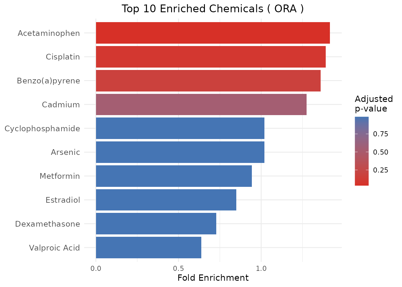
# ORA dot plot (size = gene count, color = adjusted p-value)
plot_CTD(ora_results, type = "dot", n = 10)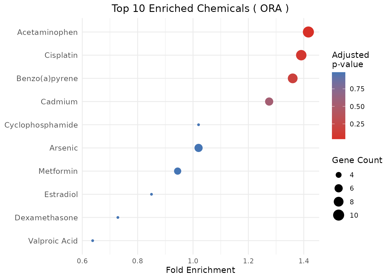
# CAMERA bar plot: x-axis = -log10(padj), fill = Direction
plot_CTD(camera_results, type = "bar")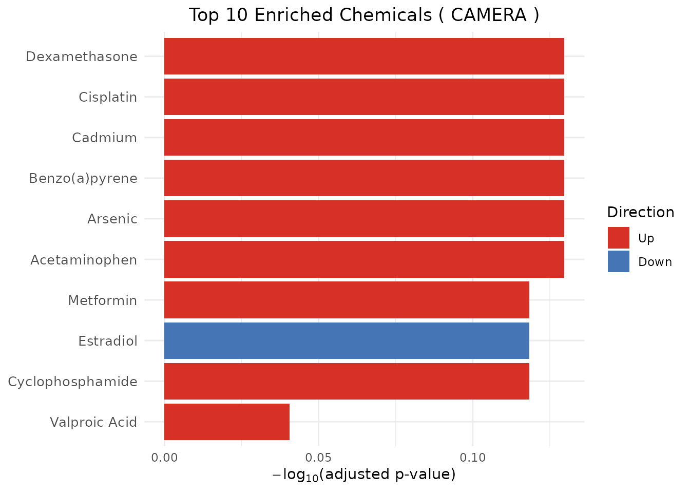
# GSVA heatmap: top-variance chemicals across samples
plot_CTD(gsva_scores)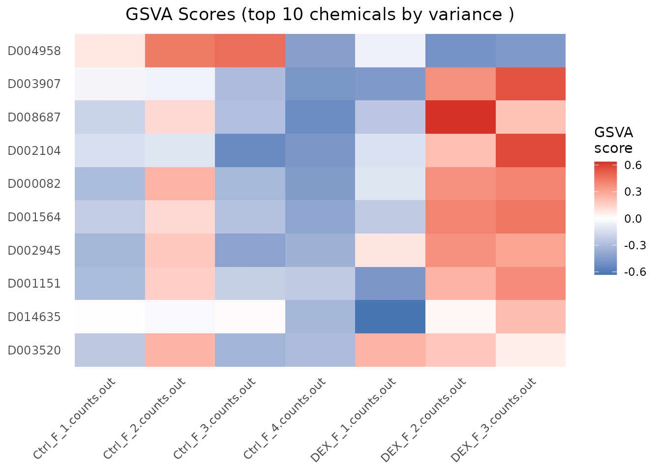
Adjusting for multiple testing
By default, enrichment_CTD() uses the Benjamini-Hochberg
("BH") method for p-value adjustment. You can change this
via the pAdjustMethod parameter:
# Bonferroni correction (more conservative)
ora_bonf <- enrichment_CTD(genes, method = "ORA",
    pAdjustMethod = "bonferroni")
#> background: all 17 genes in the CTD sets, because no 'universe' was given. If your experiment could only detect some of them, pass those as 'universe': a background wider than what was measurable makes p-values too small.

# No adjustment
ora_raw <- enrichment_CTD(genes, method = "ORA",
    pAdjustMethod = "none")
#> background: all 17 genes in the CTD sets, because no 'universe' was given. If your experiment could only detect some of them, pass those as 'universe': a background wider than what was measurable makes p-values too small.

# Compare the adjusted p-value of the top hit
data.frame(
    method = c("BH (default)", "bonferroni", "none"),
    top_padj = c(min(ora_results$padj),
        min(ora_bonf$padj), min(ora_raw$padj))
)
#> Warning in min(ora_results$padj): no non-missing arguments to min; returning
#> Inf
#> Warning in min(ora_bonf$padj): no non-missing arguments to min; returning Inf
#> Warning in min(ora_raw$padj): no non-missing arguments to min; returning Inf
#>         method top_padj
#> 1 BH (default)      Inf
#> 2   bonferroni      Inf
#> 3         none      Inf
Available methods: "BH" (default),
"bonferroni", "fdr" (alias for BH),
"none".
Gene set size filters and background universe
Each method applies a gene set size filter and defines a background universe, but the degree of user control differs:
| Method | Size filter | Configurable | Background universe | Configurable |
|---|---|---|---|---|
| ORA |
minGSSize (default 2) / maxGSSize (default
Inf) |
✓ | All genes in TERM2GENE (default) or user-supplied
universe
|
✓ |
| GSEA |
minSize / maxSize
|
✓ | No universe concept — uses the full ranked list | — |
| CAMERA | ≥ 2 genes (hard-coded) | ✗ | rownames(x) |
implicit |
| GSVA |
minSize / maxSize
|
✓ | rownames(x) |
implicit |
ORA, GSEA, and GSVA accept size-filter arguments via
..., which are forwarded to the underlying engine. CAMERA’s
minimum of 2 genes is hard-coded and cannot be changed.
The background universe is the choice that matters most
Of everything on this page, this is the argument worth getting right.
A hypergeometric test asks: drawing n genes at random from a background of N, how many would land in this chemical’s set? If N contains genes your experiment could never have detected, those genes fill the urn with balls that cannot be drawn. The overlap you observed then looks more selective than it was, and the p-value comes out too small. The error is anti-conservative: it manufactures significance rather than hiding it.
ctdR defaults to every gene in the CTD gene sets, and
says so when it does. That is a fallback, not a recommendation: the
package cannot know what your platform measured. On the RNA-seq analysis
in this package’s tutorial the difference is not subtle:
| Background | N | Chemicals significant at FDR < 0.05 |
|---|---|---|
| All CTD genes (the default) | 27,444 | 32 |
| Genes that entered the DE test | 24,845 | 19 |
Thirteen of those thirty-two are produced by the background alone. Rankings move too: benzo(a)pyrene sits fourth on the default background and tenth on the correct one.
The simpler way: hand over the whole table. Rather than filtering first and then describing the background, pass the result table and say which p-value to judge on:
enrichment_CTD(de, method = "ORA", alpha = 0.05, alpha_column = "padj")The genes below the threshold become the list to test and
every row becomes the background, the selected ones
included: the test draws n genes from an urn of N, and
the drawn genes were in the urn. The background is everything you
studied, not the non-significant remainder. Both come from one object,
so they cannot disagree. alpha_column takes a name or an
index, and naming it matters: on a table from
limma::topTable() the second column is the log fold change,
not a p-value. Which p-value to judge on is your decision, not the
package’s, and the function reports the column it used.
Or supply the background yourself, if you have already selected your genes:
enrichment_CTD(sig_genes, method = "ORA", universe = de$EntrezID)What belongs in universe is every gene that entered your
differential test. Not every gene you sequenced, and not only the
significant ones. A gene filtered out for low expression could not have
come out significant, so it does not belong in the urn either; a gene
that was tested and did not reach significance very much does.
The two are mutually exclusive: with alpha the
background is already decided.
Only ORA needs this argument, and it is worth seeing
why. The three other methods cannot get the background wrong,
because their input carries it. GSEA ranks the whole list you give it,
so the list is the background. CAMERA and GSVA intersect the gene sets
with rownames(x), so their background is the set of genes
you measured, by construction.
ORA is the exception because a bare gene list records only which
genes came out, not which ones could have. That missing information is
what universe supplies, and why its absence is the one
input error this package cannot detect for you. Passing it to GSEA,
CAMERA or GSVA raises a warning rather than being silently dropped.
Why the size thresholds are what they are
In ctdR every chemical is a gene set, and CTD
gene sets are small: the median chemical has 4 target
genes, against 72 for KEGG and 11 for GO. Size thresholds tuned for
those collections do not transfer. Measured on the full CTD
chemical-gene file, of 11,067 chemicals:
minGSSize |
Chemicals tested | % |
|---|---|---|
| 1 | 10,802 | 97.6 |
| 2 (default) | 7,970 | 72.0 |
| 3 | 6,498 | 58.7 |
| 5 | 4,844 | 43.8 |
| 10 | 2,971 | 26.8 |
A minGSSize of 10, the conventional value, would test
barely a quarter of them. The rest are not tested and found
unremarkable: they are absent from the output altogether.
One-gene sets are excluded on purpose rather than by accident. For a set of one gene the hypergeometric p-value is exactly the number of input genes divided by the background size, the same value whichever gene the set contains. It measures whether that gene is in your list, not whether the chemical is enriched. Removing those sets also makes the remaining ones easier to call significant, since they no longer add to the multiple-testing burden.
Chemicals removed by the filter are reported rather than dropped
quietly. ora() emits a message giving how many chemicals
went untested and whether they fell below or above the thresholds, so a
chemical missing from the results can be told apart from one that was
tested and came back non-significant.
Raise minGSSize when you want only well-characterised
chemicals, and lower it to 1 only if you are deliberately looking for
single-gene associations and will read those p-values accordingly.
And why there is no upper limit
The same reasoning applied to the other end reaches the opposite
answer, so maxGSSize defaults to Inf.
A set of M genes cannot, even when every one of the m input genes falls inside it, produce a p-value below C(M,m)/C(N,m), which is roughly (M/N)^m. That floor rises with M: a large enough set becomes untestable, just as a small enough one does. The question is whether CTD contains any such set.
It does not. With the 28,571 genes CTD covers and an input list of 169 differentially expressed genes, the largest still-testable set is about 26,600 genes, 93% of the universe. The largest chemical in CTD, benzo(a)pyrene, has 16,536. Every chemical in the database is testable from above, so an upper cut removes sets that could have been declared significant.
What a cut removes is also not marginal. At 500 it excludes 265 chemicals, among them benzo(a)pyrene, valproic acid, sodium arsenite, bisphenol A, aflatoxin B1 and particulate matter. Their sets are large because the literature on them is large. This is where CTD differs from GO: there a large term is one that has stopped meaning anything, here a large set is a chemical somebody has studied for decades. Keeping them costs 3% more tests, 8,235 against 7,970.
Set maxGSSize to a finite value if you have a reason of
your own, for instance to keep the focus on chemicals with sharply
defined targets. ctdR does not impose one.
What that costs, and how to read around it
Removing the cap has a consequence worth stating rather than discovering: with no upper limit, the significant results skew towards large sets. On the analysis in this vignette’s tutorial, the median chemical among the significant hits carries about 4,100 target genes, against a median of 7 across every chemical tested.
This is worth understanding rather than memorising, because the fold
enrichment appears to say the opposite. Fold is
(k/n) / (M/N): the set size M sits in the
denominator, so for a fixed overlap k a larger set gives a
lower fold. Yet larger sets reach smaller p-values.
Both are true, because the two measure different things.
The p-value does not measure the ratio. It measures how unlikely the excess is, and the excess is counted in genes, not in proportion. With 154 input genes drawn from a background of 27,444, holding the fold fixed at 1.5:
| Genes in set | Expected by chance | Observed at fold 1.5 | p |
|---|---|---|---|
| 100 | 0.6 | 1 | 0.43 |
| 2,000 | 11.2 | 17 | 0.057 |
| 16,000 | 89.8 | 135 | 1.4e-15 |
The same 50% enrichment spans fifteen orders of magnitude. A set of 100 genes at fold 1.5 is 0.4 genes above expectation, which happens constantly by chance; a set of 16,000 at the same fold is 45 genes above, which does not. The identical ratio carries incomparable evidence, and the test is right to say so.
In CTD, set size also measures how much a chemical has been studied: the database curates published literature, so a chemical measured in many genome-wide experiments accumulates many recorded genes. It is tempting to read that as a bias, and to suspect that large sets are padded with genes that respond to everything. Measured, they are not. The genes in sets above 500 appear in a median of 47 chemicals each; the genes in sets of 4 or fewer appear in a median of 232. Small sets are the ones made of the usual suspects, because a chemical studied once was studied with a targeted assay aimed at a gene somebody already suspected. Large sets are, per gene, more specific rather than less.
So finding well-studied chemicals near the top is not an artefact to be corrected. The evidence behind them is real, and no method can find a chemical nobody has measured: that is a limit of the available data, not of the test.
What it does change is what a result means, and this holds for every enrichment analysis run against a curated database, not only this one. The question the test answers is not is this chemical associated with these genes, but is this chemical associated with these genes, as far as the published literature records. Between two chemicals of equal biological relevance, the better-studied one has more opportunity to overlap your gene list and ranks higher. A chemical absent from the output is therefore uninvolved only as far as anyone currently knows: the analysis measures the state of the evidence, and reports the biology through it.
The practical consequence is how to read the output. Results are sorted by adjusted p-value, which is the quantity the false discovery rate is controlled on. Fold enrichment is not a sound sort key on its own: it has no error control, and a two-gene set with both genes hit would sit at the top of it. Read the two columns together:
| Chemical | Genes in set | Overlap | Fold | Adjusted p |
|---|---|---|---|---|
| Benzo(a)pyrene | 16,337 | 124 | 1.35 | 4.3e-05 |
| GSK-J4 | 2,331 | 35 | 2.68 | 8.0e-05 |
Both are significant, and the first ranks higher. The second is the sharper association. Neither column answers the question alone.
FoldEnrichment, Count and
BackgroundRatio are in the output for this reason. Sorting
by FoldEnrichment within the chemicals
that pass your FDR threshold is a reasonable second pass, and gives a
different and equally legitimate reading of the same result.
# ORA: restrict the background to expressed genes. Both size thresholds
# are left at their defaults; maxGSSize is shown here only to make the
# point that capping it is a deliberate choice, not a starting position.
ora_expressed <- enrichment_CTD(
    genes, method = "ORA",
    universe   = c(genes$EntrezID, "7422", "836")  # expressed genes
)

# GSEA: filter gene sets by size
gsea_filtered <- enrichment_CTD(
    genes, method = "GSEA",
    minSize = 3,
    maxSize = 300
)
#> Warning: GSEA: no 'stat' column found in input. Falling back to -log10(second
#> column) for ranking, which loses directionality and may produce ties at
#> non-significant genes. Add a signed ranking statistic (e.g. the moderated
#> t-statistic from limma::eBayes()) as a column named 'stat' to suppress this
#> warning.
#> Warning in prepareStats(stats, scoreType, gseaParam): All values in the stats
#> vector are greater than zero and scoreType is "std", maybe you should switch to
#> scoreType = "pos".
Setting universe in ORA to the full list of genes
measured in your experiment (rather than the default of all
CTD-annotated genes) is strongly recommended: it avoids inflated
fold-enrichment estimates that arise when the background is larger than
the actual measurement space.
Choosing among the four methods
| Aspect | ORA | GSEA | CAMERA | GSVA |
|---|---|---|---|---|
| Input | Gene list | Ranked gene list | Expression matrix + design + contrast | Expression matrix |
| Question | Over-represented? | Cluster at extremes? | Stronger signal than rest of transcriptome (correlation-corrected)? | Per-sample chemical score |
| Output | Ranked chemicals (data.frame) | Ranked chemicals (data.frame) | Ranked chemicals (data.frame) | Chemical x sample score matrix |
| Best for | DEG lists | Exploratory, ranked | Multi-sample DE experiments, co-regulated gene sets | Patient stratification, downstream tests, heatmaps |
Use ORA when you have a well-defined gene list above a significance threshold; GSEA to leverage the full ranking without a cutoff; CAMERA when you have a proper multi-sample design and want to control the inflated false-positive rate that ORA/GSEA exhibit on strongly co-regulated gene sets; GSVA when you want a per-sample score to feed into downstream analyses (clustering, survival, correlation with phenotypes).
Interoperability with existing Bioconductor infrastructure
ctdR’s contribution is the CTD chemical-gene sets and a
unified interface; the statistical tests themselves are delegated to
established engines (fgsea, limma,
GSVA); ORA is a hypergeometric test computed on
stats::phyper. If you would rather run the CTD gene sets
through a different engine, ctdR exposes them directly.
Reading a CTD file the BiocIO way
Besides import_CTD() (which processes and caches the
data), a CTD file can be read into memory using the standard
Bioconductor import() generic via the CTDFile
class – so the file behaves like any other BiocFile:
Handing the CTD gene sets to another engine
as_genesets_CTD() returns the chemical gene sets as a
named list, in the exact shape expected by, for example, the
gs argument of EnrichmentBrowser::sbea().
ctdR does not depend on
EnrichmentBrowser – you supply it.
gene_sets <- as_genesets_CTD("entrez")
length(gene_sets)
#> [1] 10
gene_sets[[1]]
#>  [1] "7124" "3569" "7157" "672"  "1956" "4609" "3845" "207"  "5290" "3553"
#> [11] "7422" "6774"
# Illustrative: route the CTD gene sets through EnrichmentBrowser's
# set-based engine. sbea() covers all four of ctdR's methods, GSVA
# included, plus eight more (see EnrichmentBrowser::sbeaMethods()).
library(EnrichmentBrowser)
res <- sbea(method = "camera", se = my_se, gs = as_genesets_CTD("entrez"))
gsRanking(res)
The named list is also a one-line conversion away from a
GeneSetCollection
(GSEABase::GeneSetCollection()), for tools that expect that
container.
Naming and scope: the “CTD” acronym
In ctdR, CTD always means the
Comparative Toxicogenomics Database (https://ctdbase.org). The
same acronym denotes unrelated things elsewhere in the R ecosystem: the
CRAN package CTD (“Connect The Dots”) is a graph
algorithm for metabolomic and transcriptomic perturbations, and in
EWCE a ctd object is a
CellTypeDataset. ctdR is unrelated to both. The
CTDFile class is named to avoid this collision – and to
avoid CTDData, the class of the CTD-specific package
CTDquerier, which was removed from Bioconductor at release
3.12.
Updating the CTD data
CTD releases updated data periodically. To update:
- Download the latest
CTD_chem_gene_ixns.csv.gzfrom https://ctdbase.org/reports/CTD_chem_gene_ixns.csv.gz. - Decompress and re-run
import_CTD()– existing cache files are overwritten.
import_CTD("~/Downloads/CTD_chem_gene_ixns.csv")References
ctdR supplies the CTD gene sets and a common interface;
the statistical tests are the work of others, and the methods it uses
are published. Cite the ones your analysis relied on, not the whole
list.
The data. Every result depends on the CTD release
you imported, and ctd_provenance() reports which one that
was.
- Davis AP, Wiegers TC, Johnson RJ, Sciaky D, Wiegers J, Mattingly CJ (2023). Comparative Toxicogenomics Database (CTD): update 2023. Nucleic Acids Research 51(D1), D1257-D1262. doi:[10.1093/nar/gkac833](https://doi.org/10.1093/nar/gkac833)
The methods. One reference per method, plus the implementation where it differs from the paper that introduced it.
- GSEA, the method: Subramanian A, Tamayo P, Mootha VK, et al. (2005). Gene set enrichment analysis: a knowledge-based approach for interpreting genome-wide expression profiles. PNAS 102(43), 15545-15550. doi:[10.1073/pnas.0506580102](https://doi.org/10.1073/pnas.0506580102)
-
fgsea, the implementation
ctdRcalls: Korotkevich G, Sukhov V, Budin N, Shpak B, Artyomov MN, Sergushichev A (2021). Fast gene set enrichment analysis. bioRxiv. doi:[10.1101/060012](https://doi.org/10.1101/060012) - CAMERA: Wu D, Smyth GK (2012). Camera: a competitive gene set test accounting for inter-gene correlation. Nucleic Acids Research 40(17), e133. doi:[10.1093/nar/gks461](https://doi.org/10.1093/nar/gks461)
- limma, which provides CAMERA: Ritchie ME, Phipson B, Wu D, Hu Y, Law CW, Shi W, Smyth GK (2015). limma powers differential expression analyses for RNA-sequencing and microarray studies. Nucleic Acids Research 43(7), e47. doi:[10.1093/nar/gkv007](https://doi.org/10.1093/nar/gkv007)
- GSVA: Hänzelmann S, Castelo R, Guinney J (2013). GSVA: gene set variation analysis for microarray and RNA-seq data. BMC Bioinformatics 14, 7. doi:[10.1186/1471-2105-14-7](https://doi.org/10.1186/1471-2105-14-7)
Interoperability. The compatibility section above
routes the CTD gene sets through another engine, which ctdR
does not depend on:
- Geistlinger L, Csaba G, Zimmer R (2016). Bioconductor’s EnrichmentBrowser: seamless navigation through combined results of set- & network-based enrichment analysis. BMC Bioinformatics 17, 45. doi:[10.1186/s12859-016-0884-1](https://doi.org/10.1186/s12859-016-0884-1)
The reasoning behind the size thresholds. The argument for excluding one-gene sets, and for not excluding large ones, rests on this:
- Bourgon R, Gentleman R, Huber W (2010). Independent filtering increases detection power for high-throughput experiments. PNAS 107(21), 9546-9551. doi:[10.1073/pnas.0914005107](https://doi.org/10.1073/pnas.0914005107)
The example data. The RNA-seq analysis shown here uses a subset of:
- NCBI Gene Expression Omnibus, accession GSE311566: Comparing the effects of PFAS and dexamethasone on human PBMCs (2025).
ctdR itself.
citation("ctdR") prints the current form, which includes
the version you ran and the archival DOI.
Session info
sessionInfo()
#> R version 4.6.1 (2026-06-24)
#> Platform: x86_64-pc-linux-gnu
#> Running under: Ubuntu 24.04.5 LTS
#>
#> Matrix products: default
#> BLAS:   /usr/lib/x86_64-linux-gnu/openblas-pthread/libblas.so.3
#> LAPACK: /usr/lib/x86_64-linux-gnu/openblas-pthread/libopenblasp-r0.3.26.so;  LAPACK version 3.12.0
#>
#> locale:
#>  [1] LC_CTYPE=C.UTF-8       LC_NUMERIC=C           LC_TIME=C.UTF-8
#>  [4] LC_COLLATE=C.UTF-8     LC_MONETARY=C.UTF-8    LC_MESSAGES=C.UTF-8
#>  [7] LC_PAPER=C.UTF-8       LC_NAME=C              LC_ADDRESS=C
#> [10] LC_TELEPHONE=C         LC_MEASUREMENT=C.UTF-8 LC_IDENTIFICATION=C
#>
#> time zone: UTC
#> tzcode source: system (glibc)
#>
#> attached base packages:
#> [1] stats4    stats     graphics  grDevices utils     datasets  methods
#> [8] base
#>
#> other attached packages:
#>  [1] SummarizedExperiment_1.42.0 Biobase_2.72.0
#>  [3] GenomicRanges_1.64.0        Seqinfo_1.2.0
#>  [5] IRanges_2.46.0              S4Vectors_0.50.3
#>  [7] BiocGenerics_0.58.1         generics_0.1.4
#>  [9] MatrixGenerics_1.24.0       matrixStats_1.5.0
#> [11] ctdR_0.99.11                BiocStyle_2.40.0
#>
#> loaded via a namespace (and not attached):
#>   [1] DBI_1.3.0                   httr2_1.3.0
#>   [3] GSEABase_1.74.0             rlang_1.3.0
#>   [5] magrittr_2.0.5              otel_0.2.0
#>   [7] compiler_4.6.1              RSQLite_3.53.3
#>   [9] DelayedMatrixStats_1.34.0   png_0.1-9
#>  [11] systemfonts_1.3.2           vctrs_0.7.3
#>  [13] memuse_4.2-3                SpatialExperiment_1.22.0
#>  [15] pkgconfig_2.0.3             crayon_1.5.3
#>  [17] fastmap_1.2.0               magick_2.9.1
#>  [19] dbplyr_2.6.0                XVector_0.52.0
#>  [21] labeling_0.4.3              rmarkdown_2.32
#>  [23] tzdb_0.5.0                  graph_1.90.0
#>  [25] ragg_1.5.2                  purrr_1.2.2
#>  [27] bit_4.6.0                   xfun_0.61
#>  [29] cachem_1.1.0                beachmat_2.28.0
#>  [31] jsonlite_2.0.0              blob_1.3.0
#>  [33] rhdf5filters_1.24.1         DelayedArray_0.38.2
#>  [35] Rhdf5lib_2.0.0              BiocParallel_1.46.0
#>  [37] irlba_2.4.1                 parallel_4.6.1
#>  [39] R6_2.6.1                    bslib_0.12.0
#>  [41] RColorBrewer_1.1-3          limma_3.68.5
#>  [43] jquerylib_0.1.4             Rcpp_1.1.2
#>  [45] bookdown_0.48               knitr_1.52
#>  [47] GSVA_2.6.6                  readr_2.2.0
#>  [49] Matrix_1.7-5                tidyselect_1.2.1
#>  [51] abind_1.4-8                 yaml_2.3.12
#>  [53] codetools_0.2-20            curl_8.0.0
#>  [55] lattice_0.22-9              tibble_3.3.1
#>  [57] withr_3.0.3                 KEGGREST_1.52.2
#>  [59] S7_0.2.2                    evaluate_1.0.5
#>  [61] desc_1.4.3                  BiocFileCache_3.2.0
#>  [63] Biostrings_2.80.2           pillar_1.11.1
#>  [65] BiocManager_1.30.27         filelock_1.0.3
#>  [67] vroom_1.7.1                 hms_1.1.4
#>  [69] ggplot2_4.0.3               sparseMatrixStats_1.24.0
#>  [71] scales_1.4.0                xtable_1.8-8
#>  [73] glue_1.8.1                  tools_4.6.1
#>  [75] BiocIO_1.22.0               data.table_1.18.6.1
#>  [77] ScaledMatrix_1.20.0         annotate_1.90.0
#>  [79] fgsea_1.38.0                XML_3.99-0.25
#>  [81] fs_2.1.0                    rhdf5_2.56.1
#>  [83] fastmatch_1.1-8             cowplot_1.2.0
#>  [85] grid_4.6.1                  SingleCellExperiment_1.34.0
#>  [87] AnnotationDbi_1.74.0        HDF5Array_1.40.0
#>  [89] BiocSingular_1.28.0         cli_3.6.6
#>  [91] rsvd_1.0.5                  textshaping_1.0.5
#>  [93] S4Arrays_1.12.1             dplyr_1.2.1
#>  [95] gtable_0.3.6                sass_0.4.10
#>  [97] digest_0.6.39               SparseArray_1.12.3
#>  [99] rjson_0.2.23                org.Hs.eg.db_3.23.1
#> [101] farver_2.1.2                memoise_2.0.1
#> [103] htmltools_0.5.9             pkgdown_2.2.1
#> [105] lifecycle_1.0.5             h5mread_1.4.1
#> [107] httr_1.4.9                  statmod_1.5.2
#> [109] bit64_4.8.6